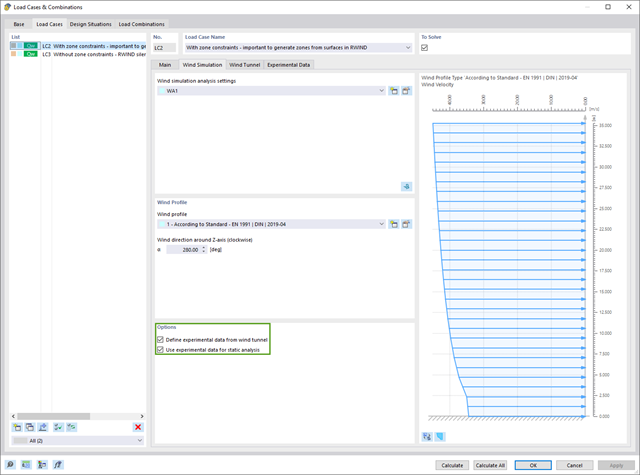
If you have experimentally determined surface pressures available for a model, you can apply them to a structural model in RFEM 6, process them in RWIND 2, and use them as wind loads in the structural analysis of RFEM 6.
You can find out how to apply the experimentally determined values in this technical article.
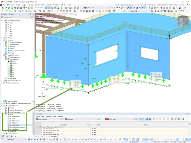
For line support results, you can optionally display certain additional information in info bubbles, such as description, sum, mean value, and so on.
If necessary, you can activate the info bubbles in the Navigator – Results.

In the Modal Analysis add-on, you have the option to automatically increase the sought eigenvalues until reaching a defined effective modal mass factor. All translational directions activated as masses for the modal analysis are taken into account.
Thus, it is possible to easily calculate the required 90% of the effective modal mass for the response spectrum method.

The modal relevance factor (MRF) can help you to assess to which extent specific elements participate in a specific mode shape. The calculation is based on the relative elastic deformation energy of each individual member.
The MRF can be used to distinguish between local and global mode shapes. If multiple individual members show significant MRF (for example, > 20%), the instability of the entire structure or a substructure is very likely. On the other hand, if the sum of all MRFs for an eigenmode is around 100%, a local stability phenomenon (for example, buckling of a single bar) can be expected.
Furthermore, the MRF can be used to determine critical loads and equivalent buckling lengths of certain members (for example, for stability design). Mode shapes for which a specific member has small MRF values (for example, < 20%) can be neglected in this context.
The MRF is displayed by mode shape in the result table under Stability Analysis → Results by Members → Effective Lengths and Critical Loads.
- Analysis of time diagrams and accelerograms (acceleration-time diagrams exciting the supports of a structure)
- Combination of user-defined time diagrams with nodal, member, and surface loads, as well as free and generated loads
- Combination of several independent excitation functions
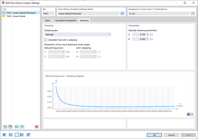
- Linear implicit Newmark analysis or modal analysis in time history
- Structural damping using Raleigh damping coefficients or Lehr's damping value
- Graphical display of results in calculation diagrams
- Result display in individual time steps or as an envelope during the entire time period
- Extensive library of seismic events (accelerograms)
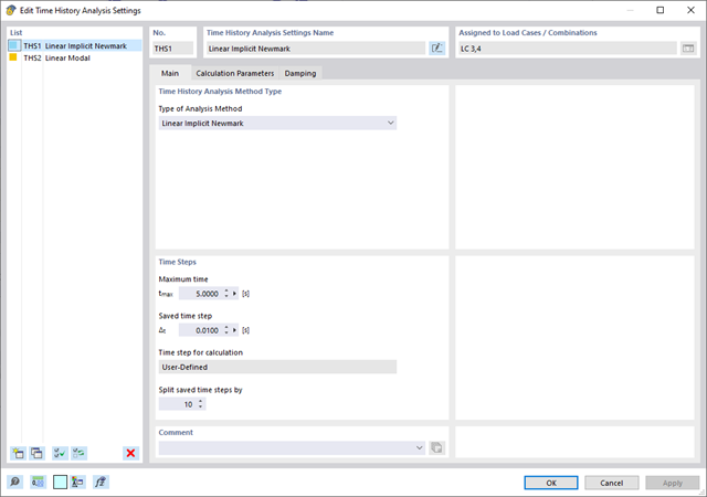
The time history analysis is performed with the modal analysis or the linear implicit Newmark analysis. The time history analysis in this add-on is limited to linear structural systems. Although the modal analysis represents a fast algorithm, it is necessary to use a certain number of eigenvalues to ensure the required accuracy of results.
The implicit Newmark analysis is a very precise method, independent of the number of eigenvalues used, but requires sufficient small time steps for the calculation.
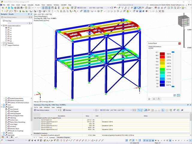
As soon as the program has completed the calculation, the summary of the results is listed. All result windows are integrated in the main program RFEM/RSTAB. You will find all the results arranged in tables; they can be displayed for each individual time step or as an envelope, and you also have the option of displaying the results graphically as well as animating them.
The results from the time history analysis can be displayed in the calculation diagrams. All the results are shown as a function of time. You can export the numeric values to MS Excel.
All result tables and graphics are part of the RFEM/RSTAB printout report. In this way, you can ensure clearly arranged documentation. You can also export the tables to MS Excel.

The Concrete Design add-on allows you to perform the seismic design of reinforced concrete members according to EC 8. This includes, among other things, the following functionalities:
- Seismic design configurations
- Differentiation of the ductility classes DCL, DCM, DCH
- Option to transfer the behavior factor from a dynamic analysis
- Check of the limit value for the behavior factor
- Capacity design checks of "Strong column - weak beam"
- Detailing and particular rules for curvature ductility factor
- Detailing and particular rules for local ductility
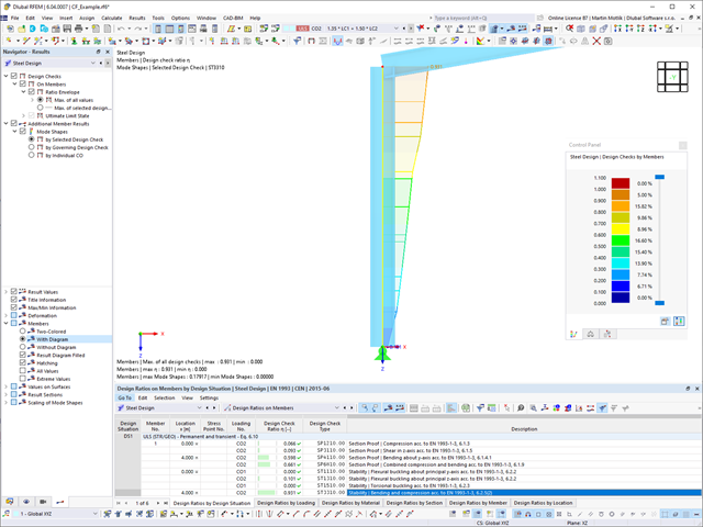
In the Steel Design add-on, you can apply a value for cold-formed sections according to EN 1993‑1‑3, which performs the stability analysis and cross-section design according to Sections 6.1.2 - 6.1.5 and 6.1.8 - 6.1.10.
Go to Explanatory Video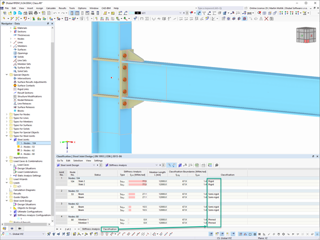
In the Steel Joints add-on, you can classify the joint stiffness.
In addition to the initial stiffness, the table also shows the limit values for hinged and rigid connections for the selected internal forces N, My, and/or Mz. The resulting classification is then displayed in tables as "hinged", "semi-rigid", or "rigid".
Go to Explanatory Video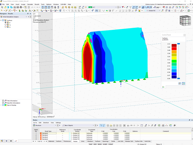
You can display the RWIND results directly in the main program. In the Navigator - Results, select the Wind Simulation Analysis result type from the list above.
Currently, the following results are available, which refer to the RWIND computational mesh:
- Surface pressure
- Surface cp coefficient
- Wall distance y+ (steady flow)
- Consideration of nonlinear component behavior using plastic standard hinges for steel (FEMA 356, EN 1998‑3) and nonlinear material behavior (masonry, steel - bilinear, user-defined working curves)
- Direct import of masses from load cases or combinations for the application of constant vertical loads
- User-defined specifications for the consideration of horizontal loads (standardized to a mode shape or uniformly distributed over the height of the masses)
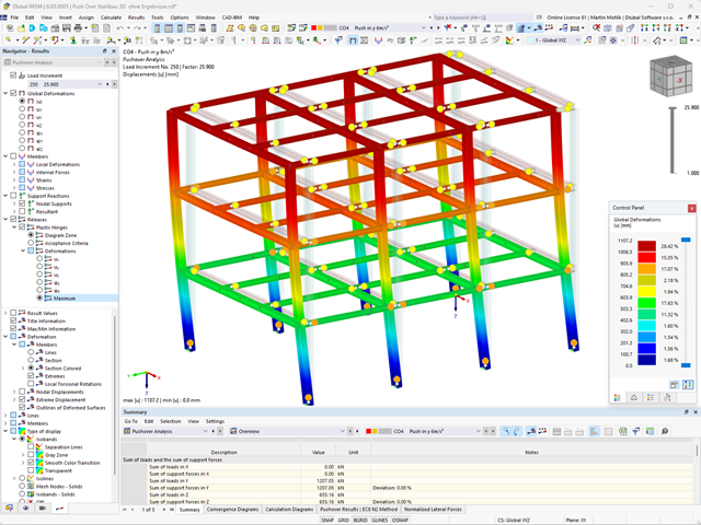
- Determination of a pushover curve with selectable limit criterion of the calculation (a collapse or limit deformation)
- Transformation of the pushover curve into the capacity spectrum (ADRS format, single degree of freedom system)
- Bilinearization of the capacity spectrum according to EN 1998‑1:2010 + A1:2013
- Transformation of the applied response spectrum into the required spectrum (ADRS format)
- Determination of target displacement according to EC 8 (the N2 method according to Fajfar 2000)
- Graphical comparison of the capacity and required spectrum
- Graphical evaluation of the acceptance criteria of predefined plastic hinges
- Result display of the values used in the iterative calculation of the target displacement
- Access to all results of the structural analysis in the individual load levels
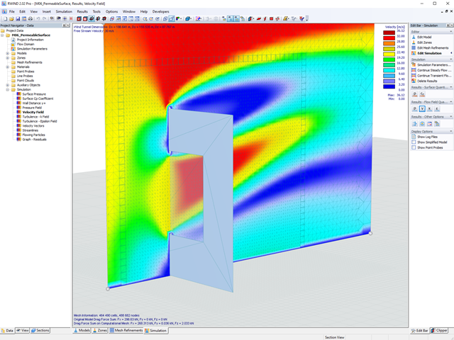
Use RWIND 2 Pro to easily apply a permeability to a surface. All you need is the definition of
- the Darcy coefficient D,
- the inertial coefficient I, and
- the length of the porous medium in the direction of flow L,
to define a pressure boundary condition between the front and back of a porous zone. Due to this setting, you obtain the flow through this zone with a two-part result display on both sides of the zone area.
But that's not all. Furthermore, the generation of a simplified model recognizes permeable zones and takes into account the corresponding openings in the model coating. Can you waive an elaborate geometric modeling of the porous element? Understandable – we have good news for you then! With a pure definition of the permeability parameters, you can avoid complex geometric modeling of the porous element. Use this feature to simulate permeable scaffolding, dust curtains, mesh structures, and so on.
More Information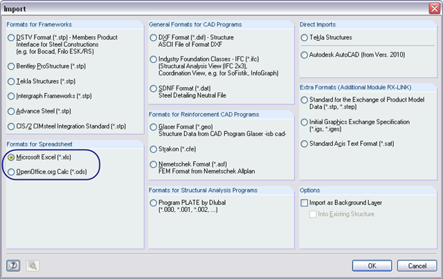
You can import table values from a prepared Excel table into RFEM 6 / RSTAB 9 with just a few clicks – either individually or all at once. For the import, you need to install a plug-in in Microsoft Excel according to this FAQ.
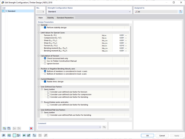
Is there torsion? In this case, you can decide how to perform the design. You have the following options:
- Allow further design if shear stress due to torsion does not exceed limit value
- Design according to Timber Construction Manual, 4.6
- Ignoring torsion
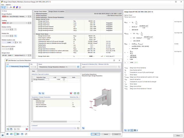
You know for sure that when connecting tension-loaded components with bolted connections, you need to consider the cross-section reduction due to the bolt holes in the ultimate limit state design. The structural analysis programs also have a solution for this. In the Aluminum Design add-on, you can enter a member local section reduction for this. Enter the reduction of the cross-section as an absolute value or as a percentage of the total area at all relevant locations.
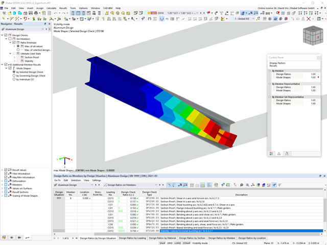
Did you use the eigenvalue solver of the add-on to determine the critical load factor within the stability analysis? In this case, you can then display the governing mode shape of the object to be designed as a result.
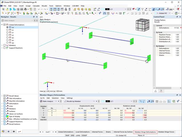
The results for members can be displayed graphically, using the Member Hinges navigator category. The numerical results of member hinges can be found in the Results by Member table category. The Member Hinge Deformations and Member Hinge Forces tables are available for the analysis and documentation of the deformation and force results in the area of member hinges.
The table lists the deformations and forces of each member for the locations specified in the Results Table Manager. There, you can also control which extreme values are displayed.
- Calculation of deflections and comparison with the normative or manually adjusted limit values
- Consideration of a precamber for the deflection analysis
- Different limit values are possible, depending on the design situation type
- Manual Adjustment of Reference Lengths and Segmentation by Direction
- Calculation of deflections related to the initial structure or to the deformed structure
- Further detailed design checks depending on the selected design standard (for example, vibration design according to EN 1999‑1‑1, 7.2.3)
- Graphical result display integrated in RFEM/RSTAB; for example, the design ratio of a limit value, or the deformation or the sag
- Complete integration of the results into the RFEM/RSTAB printout report
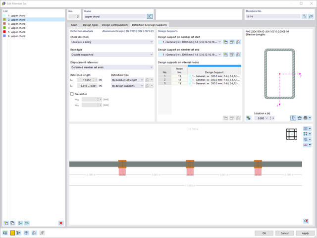
The program does a lot of work for you. For example, the load or result combinations required for the serviceability limit state are generated and calculated in RFEM/RSTAB. You can select these design situations for the deflection analysis in the Aluminum Design add-on. Depending on the specified precamber and reference system, the program determines the deformation values at each location of a member. They are then compared to the limit values.
You can specify the deformation limit value individually for each structural component in Serviceability Configuration. In this case, you define the maximum deformation depending on the reference length as the allowable limit value. By defining design supports, you can segment the components. In this way, you can determine the corresponding reference length automatically for each design direction.
And that's not all. Based on the position of the assigned design supports, the program allows you to automatically determine the distinction between beams and cantilevers. The limit value is thus determined accordingly.
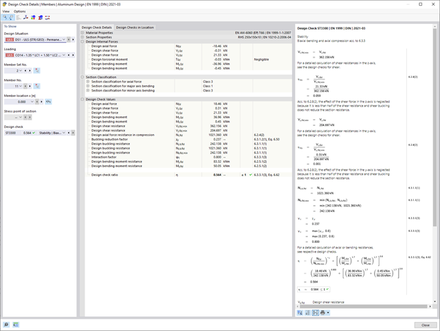
Do you prefer it clear? So do we! That's why all performed design checks for the design standard are displayed for you in a clear way. You determine a design criterion for each design check. You get design details, which include the initial values, intermediate results, and final results, arranged in a structured way for each design check. You can find the calculation process with the applied formulas, standard sources, and results in great detail in an information window in the design details.

As you've already learned, the results of a Modal Analysis load case are displayed in the program after a successful calculation. You can thus immediately see the first mode shape graphically or as an animation. You can also easily adjust the representation of the mode shape standardization. Do that directly in the Results navigator, where you have one of four options for the visualization of the mode shapes available for the selection:
- Scaling the value of the mode shape vector uj to 1 (considers the translation components only)
- Selecting the maximum translational component of the eigenvector and setting it to 1
- Considering the entire eigenvector (including the rotation components), selecting the maximum, and setting it to 1
- Setting the modal mass mi for each mode shape to 1 kg
You can find a detailed explanation of the mode shape standardization in the OnlineManual here.
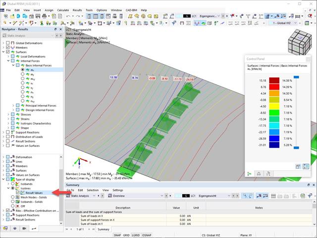
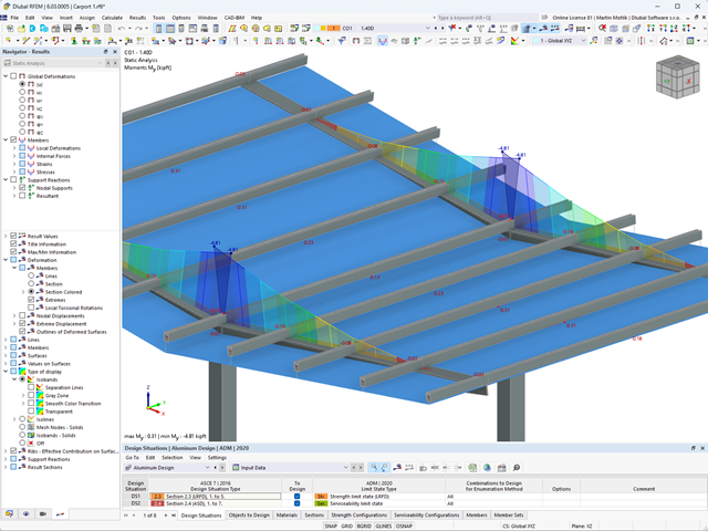
Result values for deformations, internal forces, stresses, and so on, can be displayed on the isolines.
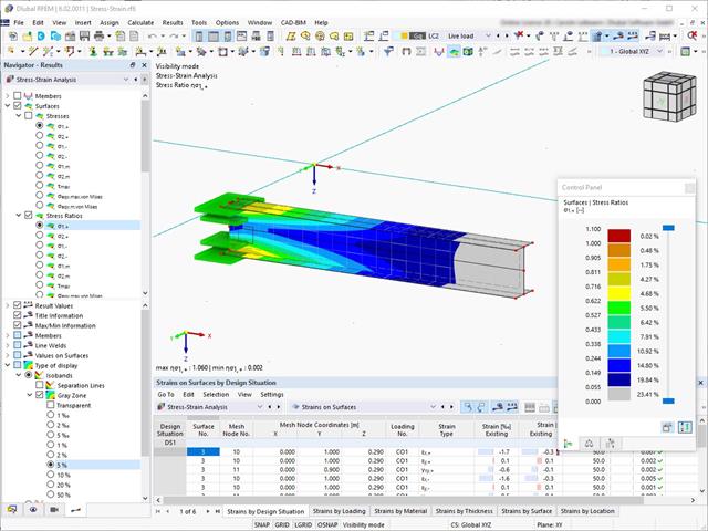
For stress-strain analyses, it is possible to define gray zones for nonrelevant value ranges in the result panel.

Is the calculation finished? The results of the modal analysis are then available both graphically and in tables. Display the result tables for the load case or the load cases of the modal analysis. Thus, you can see the eigenvalues, angular frequencies, natural frequencies, and natural periods of the structure at first glance. The effective modal masses, modal mass factors, and participation factors are also clearly displayed.
- Stability analyses for flexural buckling, torsional buckling, and flexural-torsional buckling under compression
- Import of the effective lengths from the calculation using the Structure Stability add-on
- Graphical input and check of the defined nodal supports and effective lengths for stability analysis
- Determination of the equivalent member lengths for tapered members
- Consideration of Lateral-Torsional Bracing Position
- Lateral-torsional buckling analysis of the structural components subjected to moment loading
- Depending on the standard, a choice between user-defined input of Mcr, analytical method from the standard, and use of internal eigenvalue solver
- Consideration of a shear panel and a rotational restraint when using the eigenvalue solver
- Graphical display of a mode shape if the eigenvalue solver was used
- Stability analysis of structural components with the combined compression and bending stress, depending on the design standard
- Comprehensible calculation of all necessary coefficients, such as the factors for considering moment distribution or interaction factors
- Alternative consideration of all effects for the stability analysis when determining internal forces in RFEM/RSTAB (second-order analysis, imperfections, stiffness reduction, possibly in combination with the Torsional Warping (7 DOF) add-on)
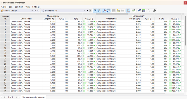
Your options in timber design are diverse. You can consider cut-to-grain angles, transverse tension stresses, and volume-dependent radii of curvature for tapered and curved members. To design the area of the grain cut, the strength is adjusted accordingly in the case of bending tension or bending pressure. In order to also allow you to perform a stability analysis with the equivalent member method, the height to determine the effective and lateral-torsional buckling lengths is set at a distance of 0.65 × h to the actual design point.
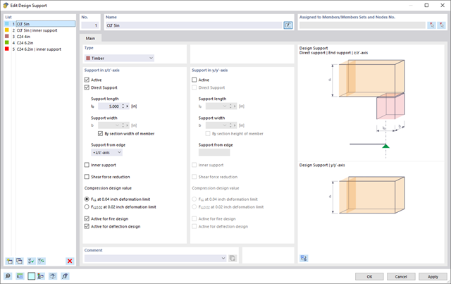
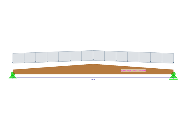
Here you have a free choice. You can perform the support pressure design at any point for the loading in the y- and z-directions of a cross-section. You are free to differentiate between inner and outer supports. A factor kc,90 for the pressure perpendicular to the grain can be user-defined (for example, 1.75 for glued-laminated timber). If allowed, the support length is increased automatically according to the standard specifications. This allows you to achieve a more efficient design with minimum effort.
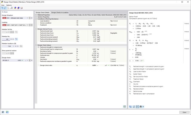
Dlubal Software just makes everything a little easier. The performed design checks of the design standard are displayed in a clear way. A design criterion is determined for each design check. Furthermore, the program deliver the design details displayed in a structured way, including the initial values, the intermediate results, and the final results. An information window in the design details shows you the calculation process with the applied formulas, standard sources, and results in great detail.
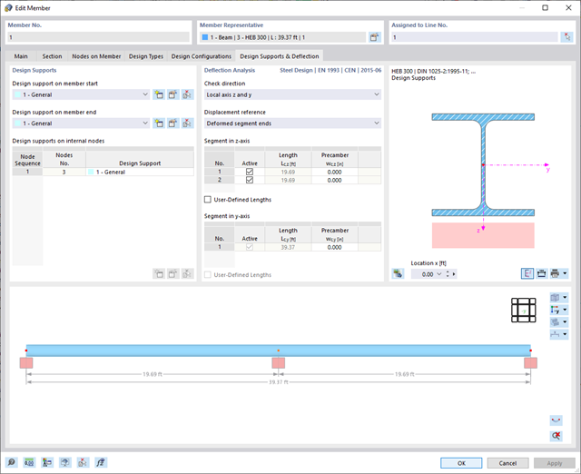
Did you know? You can individually define the reference lengths to be considered in the calculation of the deflection limit value and the segments to be checked, depending on the direction. For this, define design supports at the intermediate nodes of a member and assign them to the respective direction for the deformation analysis. In the resulting segments, you can also define a precamber for each direction and segment.